Sankey diagram maker for Windows
Turn Excel or CSV data into a Sankey chart that shows where money, energy or materials go. Make the biggest flows easy to compare, then export a clear diagram for your report or presentation.
Use one row per connection or map complete routes across stages. Keep the data, labels, units and colors together in an editable project.
For Windows 10 and Windows 11
See current price and license terms in Microsoft Store.
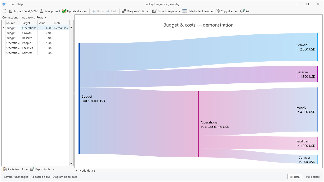
What a Sankey diagram tells you
A Sankey diagram connects categories with bands whose widths represent their values. Wider bands make the largest contributions and losses visible at a glance. Use the same unit throughout the model, such as kWh, USD or tonnes.
Use it for an energy balance, a budget breakdown, material flows or routes through a process. For a schedule with task dates, a Gantt chart is a better fit.
From spreadsheet rows to a story people can follow
1. Bring in your data
Import Excel or CSV, paste a table, or add rows yourself. Review the mapping and validation before the data enters your diagram.
2. Make the flow clear
Choose the stages, show values and units, and keep node colors consistent. Filter the table to focus the discussion.
3. Share the result
Export PNG, SVG or PDF for a presentation or report. Save the editable project so you can return to the data and appearance.
Choose the input that fits your data
One row per connection
Use Source, Target and Value when you already know each link. Build a budget breakdown or a flow model with explicit inputs, outputs and losses.
One row per complete route
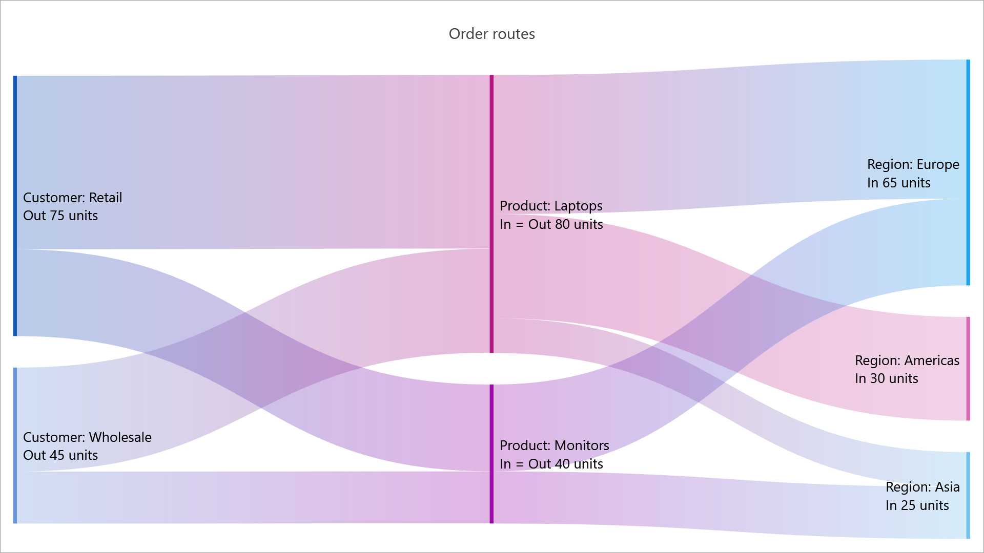
Map two to six stage columns, such as Customer → Product → Region. Keep the original records and notes, then compare the sum of a value with the number of records.
A repeatable report
Remember a local Excel or CSV file and manually reload its saved data. Review the replacement before applying it; Undo can restore your previous working table.
Make everyday analysis easier
Read the numbers in context
Show incoming and outgoing node values, apply a unit and choose decimal precision. Link tooltips help compare a connection with its source and target.
Keep the picture consistent
Choose a palette, set individual node colors and rename categories throughout the data. Appearance settings stay with the project.
Focus on the relevant flows
Filter the table and see which data is included. The diagram and export follow the same view; All data returns to the full table.
Stay in control of Excel updates
Import a one-time copy or remember a file for later reloads. Save project keeps your .sad file; it never sends edits back to Excel.
Revise with confidence
Undo and Redo support editing, imports, mapping and appearance changes. Save editable projects and recover available periodic copies after an interruption.
Export for your audience
Create presentation-size PNG images, vector SVGs or printable PDFs. Copy a diagram to the clipboard or export the visible table separately.
How to make a Sankey diagram from Excel
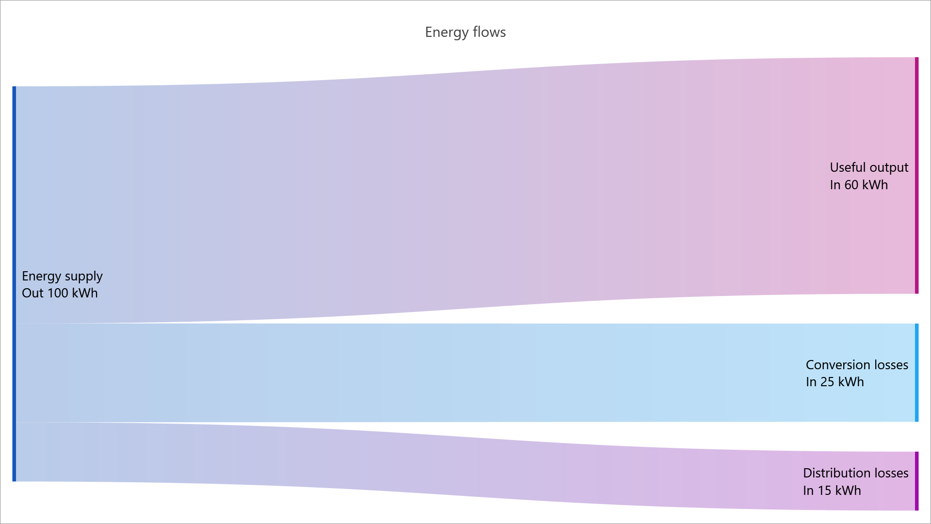
Start with three columns: Source, Target and Value. Each row describes one connection. In this fictional energy balance, 100 kWh is divided into useful output and two kinds of loss.
| Source | Target | Value |
|---|---|---|
| Energy supply | Useful output | 60 |
| Energy supply | Conversion losses | 25 |
| Energy supply | Distribution losses | 15 |
Use consistent category names and keep the Value cells numeric. Put the unit in the diagram settings, rather than adding “kWh” to each spreadsheet cell.
- Choose Import Excel / CSV and open the workbook. Select its worksheet and check whether the first row contains headers.
- Choose Connections, map Source, Target and Value, and check the number format. Note is optional.
- Choose Preview data, review the rows and import. Then choose Update diagram.
- Use Diagram Options for the title, values and kWh unit. Save the editable .sad project and export the picture separately.
Read the result before you share it
Useful output accounts for 60% of the original input. Conversion losses account for 25%, and distribution losses for 15%. The three destinations add back to 100 kWh.
Save the .sad project to keep editing. Choose Export diagram → PNG image for a presentation image, SVG vector image for scalable artwork, or PDF document for a report.
Watch the complete first-diagram tutorial or download the practice workbooks and finished examples.
This written example keeps the workbook’s original 60 / 25 / 15 values. The video also demonstrates editing them to 65 / 20 / 15 after import.
Follow the same flow through another stage
A category can receive a flow in one row and send it onward in another. Split the 60 kWh of Useful output into Service A (45) and Service B (15), using the exact same “Useful output” name in Source and Target.
| Source | Target | Value |
|---|---|---|
| Useful output | Service A | 45 |
| Useful output | Service B | 15 |
The five connection values add to 160, but the original input remains 100 kWh. The 60 passing through Useful output is counted at two transitions. Compare the inputs, final destinations and values at each node; do not treat the sum of every band as an overall total.
If each row already describes a whole route, use Records across stages instead. It builds the adjacent connections while keeping your original table.
See Sankey Diagram in action
Three short tutorials take you from your first import to recurring reports and records across stages.
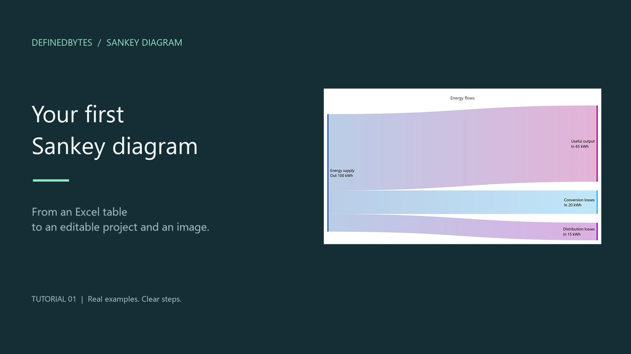
Create your first diagram from Excel
2:34 · English
Import a flow table, correct values, add readable labels, and save both an editable project and a presentation image.
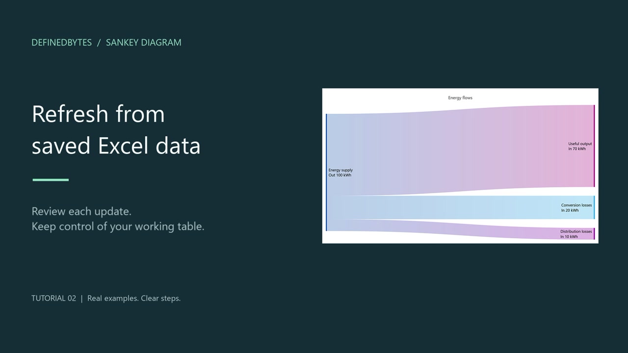
Refresh a report from saved Excel data
2:30 · English
Remember a source workbook, review its saved changes, and refresh the report while keeping the title and appearance.
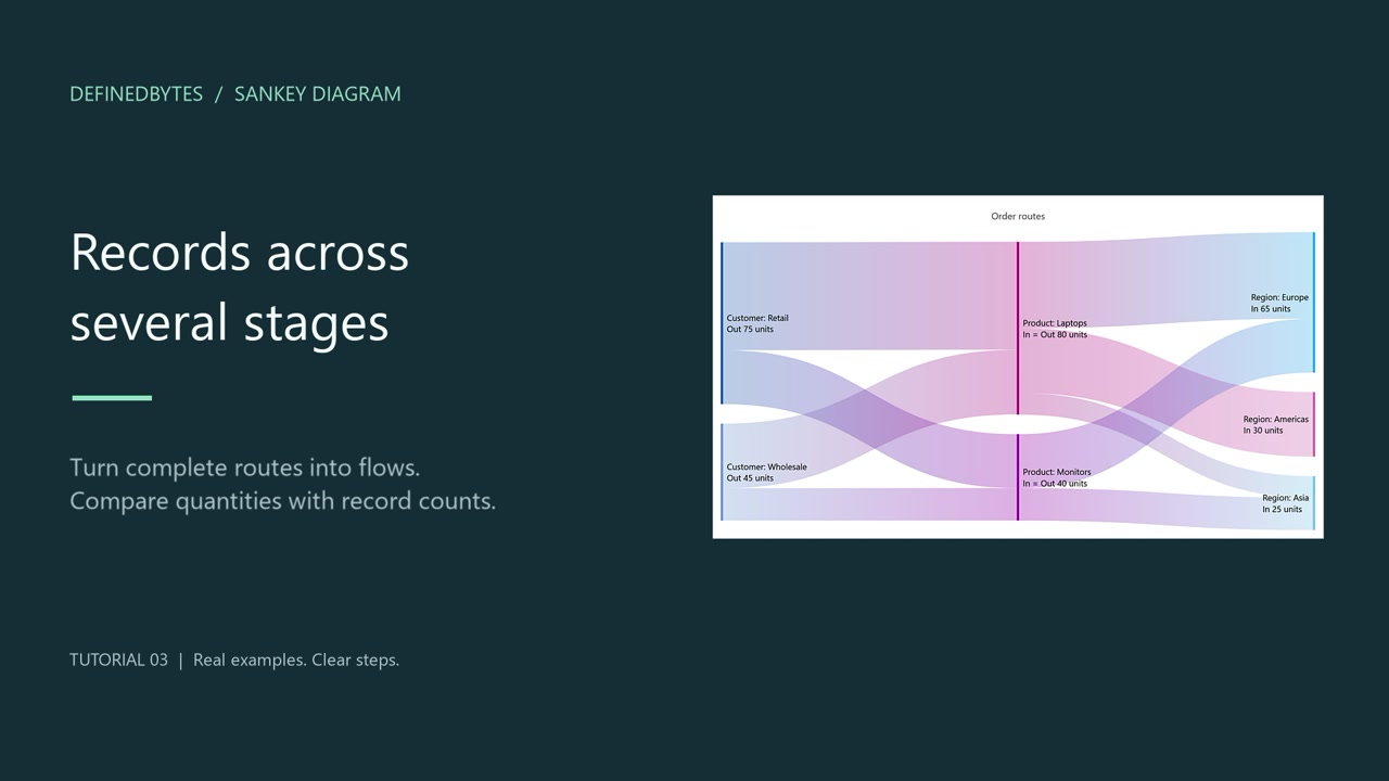
Build routes across stages: Sum or Count
2:38 · English
Map Customer, Product and Region, keep the original records editable, and compare quantities with the number of records.
Common questions
Should I choose Connections or Records across stages?
Connections uses one row per Source → Target link, with a numeric Value and optional Note. Choose it when your table already lists the connections.
Records across stages uses one row per complete route, such as Customer → Product → Region. Choose two to six ordered stage columns, then either sum a numeric column or count the records. All original columns remain available in the table.
How do Import, Reload and Save project differ?
Import copies data into your working table. Enable Remember this file for future reloads if you want to read that file again later. Reload from source reads the saved file when you request it and lets you review the replacement. Save project stores your editable .sad project.
Changes made in Sankey are not written back to Excel or CSV. There is no two-way or automatic synchronization.
Should I save a project or export a diagram?
Use Save project to keep editable data, notes and presentation settings in a .sad file. Use Export diagram for PNG, SVG or PDF to share the finished picture. Export table separately writes the visible table to XLSX, XLS, CSV or TXT.
Saving a project or exporting a table does not overwrite a connected source workbook.
Make your next flow easier to understand
Bring in the data, make the relationships clear, and share a diagram your audience can follow.
For Windows 10 and Windows 11. See current price and license terms in Microsoft Store.